机器学习：对数几率回归-2

通过上一篇文章我们可以了解到，对数几率回归是什么，相关公式的定义以及训练使用的学习方法，希望读者应当首先通过上一篇文章来了解什么是对数几率回归。这一篇文章我想写一下关于二元的对数几率回归的内容，相关的知识可以推广到多元的对数几率回归。二元乃至多元的模型就初步有了神经网络的感觉，当然，此时仍然没有隐藏层。二元的模型常常是用来做平面的数据分类的，因此我打算用一个我定义的二元数据来解释一下这个模型。

首先，我定义（即为所收集数据的实际模型）为X+Y<1的为0类即反例，否则为1类即正例，其中，个别数据允许有错误。那么，我们可以有如下数据：

X1	1	0.5	0.4	-1	-0.5	-0.5	0.5	0.5	0	0	2	1.5	1.5	0.5	1.2	0.8
X2	2	1.5	2	0	-0.5	0.5	-0.5	0	0.5	0	0.4	0	1.5	0.4	1.5	0.7
Y	1	1	1	0	0	0	0	0	0	0	1	1	1	0	1	1

在上一篇文章中，我们的数据是单变量的，所以数据读入之后它是一个列向量，而在本文中，每一组数据包含2个变量，有16组数据，所以最终输入时是16*2的矩阵，当然，对应的标记Y仍然是一个列向量。

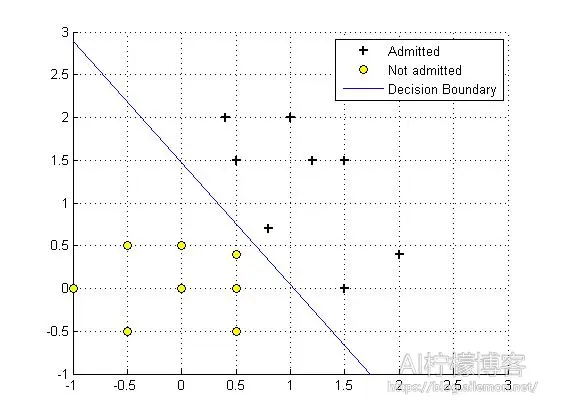
同样，我们仍然使用Sigmoid函数来作为拟合函数，代价函数和梯度的定义还是一样的，梯度下降时参数theta的迭代公式也不变。我们继续分别使用最小化函数fminunc()和自实现的梯度下降来进行机器学习训练。本篇的重点在于理解如何从单变量的统计回归模型推广到多变量模型中去，一旦理解了这一点，我们就可以将其推广到任意维度。

经过训练，我们可以得到结果：

fminunc函数：

theta =

-24.8399
24.0879
16.8938

cost =

3.7364e-04

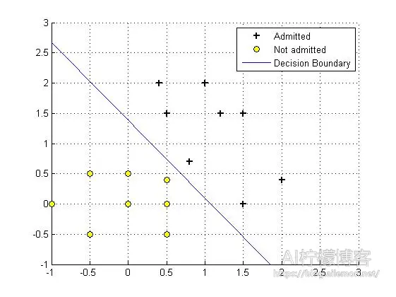
梯度下降自实现：

theta =

-23.4586
21.8901
17.0033

cost =

3.7364e-04

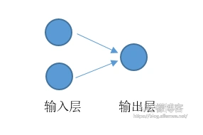
本例中，该对数几率回归模型可以看作输入层有两个神经元输出层一个神经元并且没有隐含层的神经网络，同上篇文章一样，我省去了偏置神经元（即常数项）。

MATLAB代码：

sigmoid.m

function g = sigmoid(z)
%计算sigmoid函数值
g = zeros(size(z));
g=1./(1+exp(-1.*z));
end

CostFunction.m

function [J, grad] = CostFunction(theta, X, y)
%计算对数几率回归的代价函数和梯度
m = length(y); % 训练样例数
J = 0;
grad = zeros(size(theta));
J = sum(-y .* log(sigmoid(X * theta)) - (1 - y) .* log(1 - sigmoid(X * theta)) )/m;
grad = (X' * (sigmoid(X * theta) - y))/m;
end

plotData.m （样例数据展示）

function plotData(X, y)
% 创建新图型
figure; hold on;
% 寻找正样例和负样例的索引
pos = find(y==1); neg = find(y == 0);
% 拟合样例
plot(X(pos, 1), X(pos, 2), 'k+','LineWidth', 2, ...
'MarkerSize', 7);
plot(X(neg, 1), X(neg, 2), 'ko', 'MarkerFaceColor', 'y', ...
'MarkerSize', 7);
hold off;
end

plotDecisionBoundary.m （拟合决策边界）

function plotDecisionBoundary(theta, X, y)
% 拟合数据
plotData(X(:,2:3), y);
hold on

if size(X, 2) <= 3
    % Only need 2 points to define a line, so choose two endpoints
    plot_x = [min(X(:,2))-2,  max(X(:,2))+2];

    % Calculate the decision boundary line
    plot_y = (-1./theta(3)).*(theta(2).*plot_x + theta(1));

    % Plot, and adjust axes for better viewing
    plot(plot_x, plot_y)
    
    % Legend, specific for the exercise
    legend('Admitted', 'Not admitted', 'Decision Boundary')
    axis([-1, 3, -1, 3])
else
    % Here is the grid range
    u = linspace(-1, 1.5, 50);
    v = linspace(-1, 1.5, 50);

    z = zeros(length(u), length(v));
    % Evaluate z = theta*x over the grid
    for i = 1:length(u)
        for j = 1:length(v)
            z(i,j) = mapFeature(u(i), v(j))*theta;
        end
    end
    z = z'; % important to transpose z before calling contour

    % Plot z = 0
    % Notice you need to specify the range [0, 0]
    contour(u, v, z, [0, 0], 'LineWidth', 2)
end
hold off
grid on
end

logistic_fmin2.m

%% 数据
X=[1 2;0.5 1.5;0.4 2;-1 0; -0.5 -0.5; -0.5 0.5; 0.5 -0.5; 0.5 0; 0 0.5; 0 0; 2 0.4; 1.5 0; 1.5 1.5; 0.5 0.4; 1.2 1.5; 0.8 0.7 ];
Y=[1 1 1 0 0 0 0 0 0 0 1 1 1 0 1 1]';
%% 初始参数配置
%  获取数据样本数量
[m, n] = size(X);
%在列向量的左边添加一列全为1的列向量
X = [ones(m, 1) X];
% 初始化拟合参数
initial_theta = zeros(n + 1, 1);
%计算并显示初始的代价和梯度
[cost, grad] = CostFunction(initial_theta, X, Y)
%% 使用fminunc()函数/自制梯度下降来最小化代价函数

%  为函数fminunc设置参数
options = optimset('GradObj', 'on', 'MaxIter', 400);
%  该函数将返回theta和cost 
[theta, cost] = fminunc(@(t)(CostFunction(t, X, Y)), initial_theta, options)

%% 数据拟合结果展示
% 拟合决策边界
plotDecisionBoundary(theta, X, Y);

theta
J_history(iterations)

logistic_grad2.m

%% 数据
X=[1 2;0.5 1.5;0.4 2;-1 0; -0.5 -0.5; -0.5 0.5; 0.5 -0.5; 0.5 0; 0 0.5; 0 0; 2 0.4; 1.5 0; 1.5 1.5; 0.5 0.4; 1.2 1.5; 0.8 0.7 ];
Y=[1 1 1 0 0 0 0 0 0 0 1 1 1 0 1 1]';

%% 初始参数配置
%  获取数据样本数量
[m, n] = size(X);
% 在列向量的左边添加一列全为1的列向量
X = [ones(m, 1) X];
% 初始化拟合参数
theta=zeros(n + 1, 1);

% 计算并显示初始的代价和梯度
[cost, grad] = CostFunction(theta, X, Y)
%% 自制梯度下降来最小化代价函数

iterations = 100000; % 设置迭代次数
alpha = 1; % 设置学习率

J_history = zeros(iterations, 1);
for iter = 1:iterations % 这里不用while的原因是一旦出现发散的情况，程序将陷入死循环
    [J_history(iter),grad] = CostFunction(theta, X, Y);
    theta = theta - alpha * grad;
end

%% 数据拟合结果展示
% 拟合决策边界
plotDecisionBoundary(theta, X, Y);

theta
J_history(iterations)

写在最后：
鉴于本人水平有限，如果文章中有什么错误之处，欢迎指正，非常感谢。

版权声明 本博客的文章除特别说明外均为原创，本人版权所有。欢迎转载，转载请注明作者及来源链接，谢谢。 本文地址: https://blog.ailemon.net/2017/02/14/machine-learning-logistic-regression-2/ All articles are under Attribution-NonCommercial-ShareAlike 4.0

Donate

WeChat DonateAlipay Donate